43 multiple data labels excel pie chart
Edit titles or data labels in a chart - support.microsoft.com To edit the contents of a title, click the chart or axis title that you want to change. To edit the contents of a data label, click two times on the data label that you want to change. The first click selects the data labels for the whole data series, and the second click selects the individual data label. Click again to place the title or data ... How to Create and Format a Pie Chart in Excel - Lifewire Select the plot area of the pie chart. Right-click the chart. Select Add Data Labels . Select Add Data Labels. In this example, the sales for each cookie is added to the slices of the pie chart. Change Colors When a chart is created in Excel, or whenever an existing chart is selected, two additional tabs are added to the ribbon.
How to Make a Pie Chart with Multiple Data in Excel (2 Ways) By following the above steps, you can easily edit the Color and Style of a Pie Chart. Formatting Data Labels. In Pie Chart, we can also format the Data Labels with some easy steps. These are given below. Steps: First, to add Data Labels, click on the Plus sign as marked in the following picture.
Multiple data labels excel pie chart
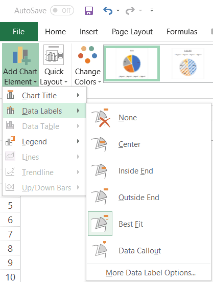
How to Create a Pie Chart in Microsoft Excel Step 3: Create the Pie Chart. To create the pie chart, go to the Insert tab in your Excel window, then click on the Pie Chart icon, which is represented as a circular button in the Chart group. After that, select the pie chart option that you want to create. This includes 2D, 3D, and doughnut pie charts. It will then create a pie chart with the ... Add or remove data labels in a chart - support.microsoft.com Click the data series or chart. To label one data point, after clicking the series, click that data point. In the upper right corner, next to the chart, click Add Chart Element > Data Labels. To change the location, click the arrow, and choose an option. If you want to show your data label inside a text bubble shape, click Data Callout. Create a multi-level category chart in Excel - ExtendOffice 2. Select the data range, click Insert > Insert Column or Bar Chart > Clustered Bar.. 3. Drag the chart border to enlarge the chart area. See the below demo. 4. Right click the bar and select Format Data Series from the right-clicking menu to open the Format Data Series pane.. Tips: You can also double click any of the bars to open the Format Data Series pane.
Multiple data labels excel pie chart. Adding second set of data labels - Excel Help Forum Re: Adding second set of data labels. The chart links to workbooks on your hard drive, not to the data in the sheet. The secondary axis can only be shown when there is a series plotting on the secondary axis. Both your series are plotted on the first axis. You need to select the COUNT OF PARTS series, format it and send it to the secondary axis. How to Explode Pie Chart in Excel (2 Easy Methods) 2. Use Format Data Series Option to Explode Pie Chart. Excel has a built-in function to explode pie chart. Here we will learn how to explode a pie chart in Excel using the built-in function with the steps below. Steps: Firstly, we need to select the pie chart and right-click on it. Secondly, select the Format Data Series option from the ... Multiple Data Labels on a Pie Chart - MrExcel Message Board #1 Hello All, So I have a table with 8 rows and 3 columns. This table includes: Column 1 - shipment name Column 2 - shipment cost Column 3 - shipment weight I have created a pie chart from this table, which covers the first two columns. Displayed next to each slice is a label with the shipment name, shipment cost, and percent share of the pie. How to Create Multi-Category Charts in Excel? - GeeksforGeeks Step 1: Insert the data into the cells in Excel. Now select all the data by dragging and then go to "Insert" and select "Insert Column or Bar Chart". A pop-down menu having 2-D and 3-D bars will occur and select "vertical bar" from it. Select the cell -> Insert -> Chart Groups -> 2-D Column Bar Chart Insertion Multi-Category Chart
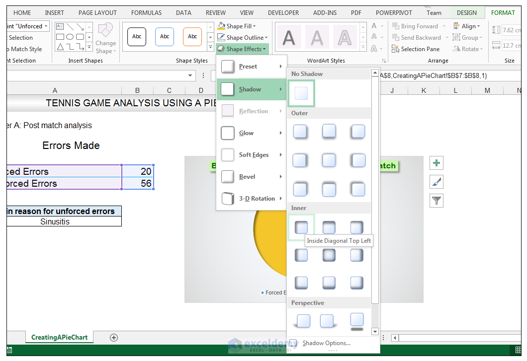
How to Combine or Group Pie Charts in Microsoft Excel Click on the first chart and then hold the Ctrl key as you click on each of the other charts to select them all. Click Format > Group > Group. All pie charts are now combined as one figure. They will move and resize as one image. Choose Different Charts to View your Data Move data labels - support.microsoft.com Click any data label once to select all of them, or double-click a specific data label you want to move. Right-click the selection > Chart Elements > Data Labels arrow, and select the placement option you want. Different options are available for different chart types. For example, you can place data labels outside of the data points in a pie ... Creating Pie Chart and Adding/Formatting Data Labels (Excel) Creating Pie Chart and Adding/Formatting Data Labels (Excel) How to Format Data Labels in Excel (with Easy Steps) Step-by-Step Procedure to Format Data Labels in Excel. Step 1: Create Chart. Step 2: Add Data Labels to Chart. Step 3: Modify Fill and Line of Data Labels. Step 4: Change Effects to Format Data Labels. Step 5: Modify Size and Properties of Data Labels. Step 6: Modify Label Options to Format Data Labels. Conclusion.
How to add data labels from different column in an Excel chart? This method will introduce a solution to add all data labels from a different column in an Excel chart at the same time. Please do as follows: 1. Right click the data series in the chart, and select Add Data Labels > Add Data Labels from the context menu to add data labels. 2. How to group (two-level) axis labels in a chart in Excel? Create a Pivot Chart with selecting the source data, and: (1) In Excel 2007 and 2010, clicking the PivotTable > PivotChart in the Tables group on the Insert Tab; (2) In Excel 2013, clicking the Pivot Chart > Pivot Chart in the Charts group on the Insert tab. 2. In the opening dialog box, check the Existing worksheet option, and then select a ... Solved: Show multiple data lables on a chart - Power BI For example, I'd like to include both the total and the percent on pie chart. Or instead of having a separate legend include the series name along with the % in a pie chart. I know they can be viewed as tool tips, but this is not sufficient for my needs. Many of my charts are copied to presentations and this added data is necessary for the end ... Formatting data labels and printing pie charts on Excel for Mac 2019 ... Here's a work around I found for printing pie charts. Still can't find a solution for formatting the data labels. 1. When printing a pie chart from Excel for mac 2019, MS instructions are to select the chart only, on the worksheet > file > print. Excel is supposed to print the chart only (not the data ) and automatically fit it onto one page.
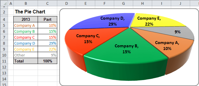
Excel 3-D Pie charts - Microsoft Excel 2010
Excel Pie Chart Labels on Slices: Add, Show & Modify Factors First of all, double-click on the data labels on the pie chart. As a result, a side window called Format Data Labels will appear. Then, go to the drop-down of the Label Options to Label Options tab. After that, check the Percentages option and uncheck all other options. You will get the percentages in the data labels.

Lesson 2 | How to Create Charts Using Microsoft Excel Tutorial
How to display leader lines in pie chart in Excel? - ExtendOffice To display leader lines in pie chart, you just need to check an option then drag the labels out. 1. Click at the chart, and right click to select Format Data Labels from context menu. 2. In the popping Format Data Labels dialog/pane, check Show Leader Lines in the Label Options section. See screenshot:

How to make a pie chart in Excel
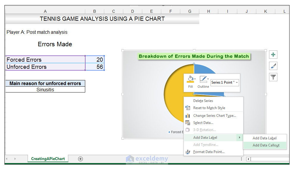
Add data labels and callouts to charts in Excel 365 | EasyTweaks.com Step #1: After generating the chart in Excel, right-click anywhere within the chart and select Add labels . Note that you can also select the very handy option of Adding data Callouts. Step #2: When you select the "Add Labels" option, all the different portions of the chart will automatically take on the corresponding values in the table ...

Excel 3-D Pie Charts - Microsoft Excel undefined
Change the format of data labels in a chart To get there, after adding your data labels, select the data label to format, and then click Chart Elements > Data Labels > More Options. To go to the appropriate area, click one of the four icons ( Fill & Line, Effects, Size & Properties ( Layout & Properties in Outlook or Word), or Label Options) shown here.

How to Create a Pie Chart in Microsoft Excel
Select all Data Labels at once - Microsoft Community AFAIK it has never been possible to select all data labels (if there are multiple series) You might be able to use code like this. Sub DL () Dim ocht As Chart Dim ser As Series Dim opt As Point Dim s As Long Dim p As Long Set ocht = ActiveWindow.Selection.ShapeRange (1).Chart For s = 1 To ocht.SeriesCollection.Count
How to Make a Pie Chart in Excel & Add Rich Data Labels to The Chart!
Quickly create multiple progress pie charts in one graph 1. Click Kutools > Charts > Difference Comparison > Progress Pie Chart to go to the Progress Pie Chart dialog box. 2. In the popped out dialog box, select the data range of the axis labels, actual values and target values under the Axis Labels, Actual Value and Target Value boxes separately. See screenshot:

How to Make Pie Charts and Graphs in Excel - BSUPERIOR
How to Make Multiple Pie Charts from One Table (3 Easy Ways) Afterward, go to the Insert tab >> click on Pie Charts. Then, select the 2-D Pie chart. After that, click on the "+" sign to open Chart Elements. Next, turn on Data Labels. Finally, you will get one pie chart from multiple tables in Excel. Practice Section
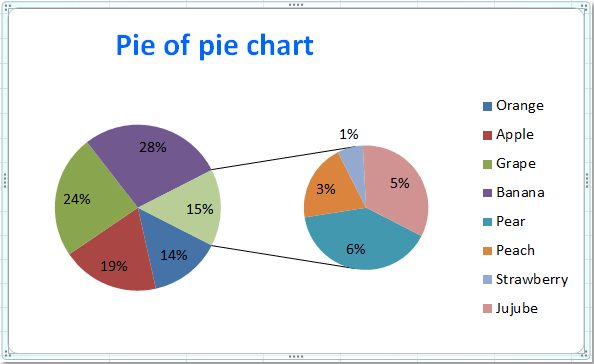
How to create pie of pie or bar of pie chart in Excel?
Pie Chart in Excel | How to Create Pie Chart - EDUCBA Step 1: Select the data to go to Insert, click on PIE, and select 3-D pie chart. Step 2: Now, it instantly creates the 3-D pie chart for you. Step 3: Right-click on the pie and select Add Data Labels. This will add all the values we are showing on the slices of the pie.

How to Make a PIE Chart in Excel (Easy Step-by-Step Guide)
Multiple data labels (in separate locations on chart) Re: Multiple data labels (in separate locations on chart) You can do it in a single chart. Create the chart so it has 2 columns of data. At first only the 1 column of data will be displayed. Move that series to the secondary axis. You can now apply different data labels to each series. Attached Files 819208.xlsx (13.8 KB, 265 views) Download

Line Chart in Excel - Easy Excel Tutorial
Create a multi-level category chart in Excel - ExtendOffice 2. Select the data range, click Insert > Insert Column or Bar Chart > Clustered Bar.. 3. Drag the chart border to enlarge the chart area. See the below demo. 4. Right click the bar and select Format Data Series from the right-clicking menu to open the Format Data Series pane.. Tips: You can also double click any of the bars to open the Format Data Series pane.
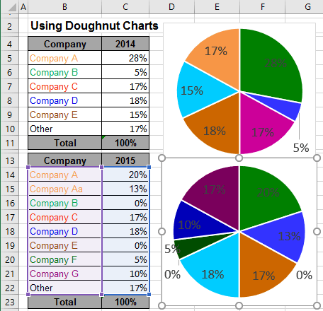
Using Pie Charts and Doughnut Charts in Excel
Add or remove data labels in a chart - support.microsoft.com Click the data series or chart. To label one data point, after clicking the series, click that data point. In the upper right corner, next to the chart, click Add Chart Element > Data Labels. To change the location, click the arrow, and choose an option. If you want to show your data label inside a text bubble shape, click Data Callout.
How to Make a PIE Chart in Excel (Easy Step-by-Step Guide)
How to Create a Pie Chart in Microsoft Excel Step 3: Create the Pie Chart. To create the pie chart, go to the Insert tab in your Excel window, then click on the Pie Chart icon, which is represented as a circular button in the Chart group. After that, select the pie chart option that you want to create. This includes 2D, 3D, and doughnut pie charts. It will then create a pie chart with the ...

New, better alternative to Pie Charts: Treemap - Efficiency 365
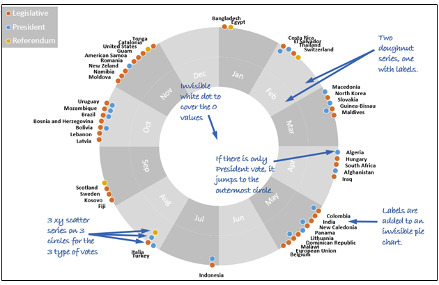
Combine pie and xy scatter charts - Advanced Excel Charting Example
How to Make a Pie Chart in Excel & Add Rich Data Labels to The Chart!
Excel charts: add title, customize chart axis, legend and data labels

How to make a pie chart in Excel
Post a Comment for "43 multiple data labels excel pie chart"